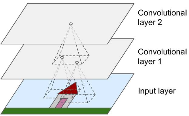
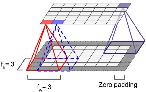
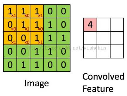
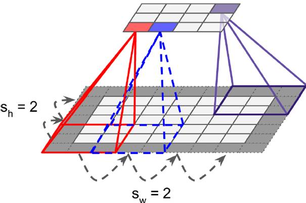
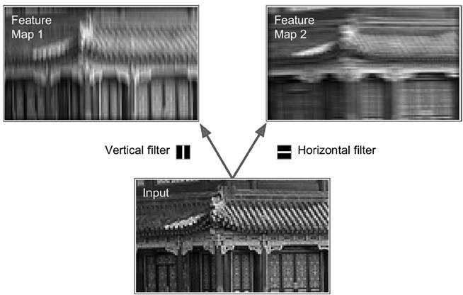
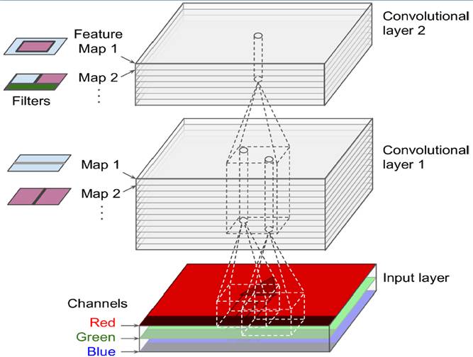
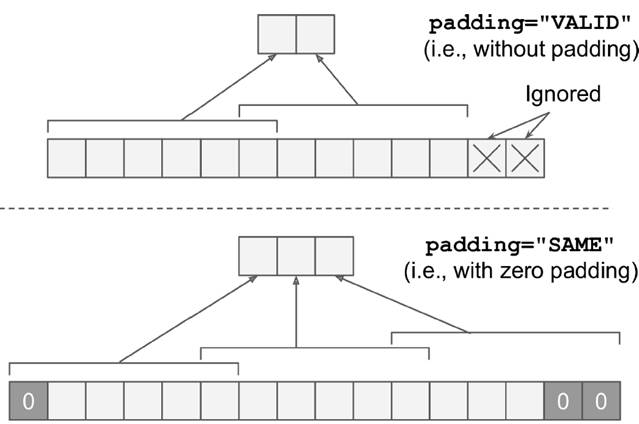
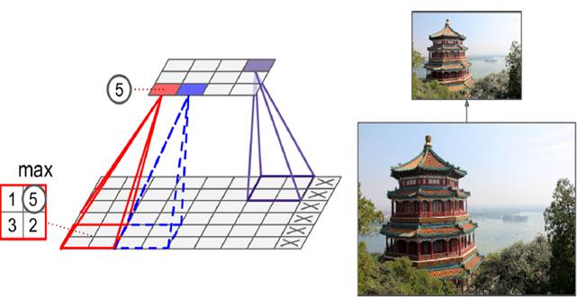
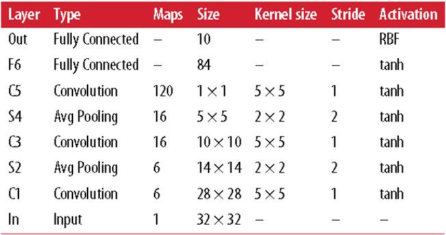
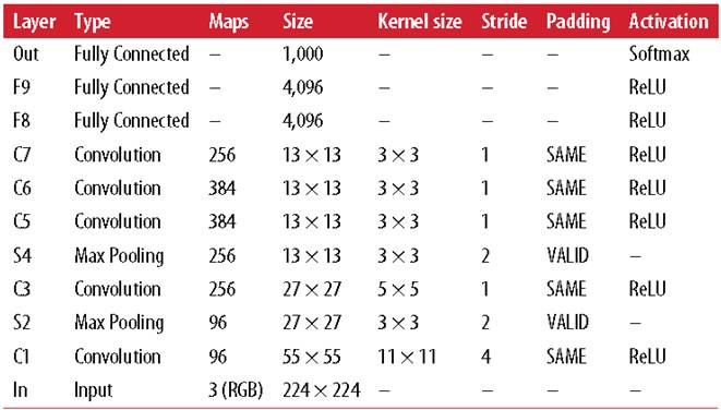
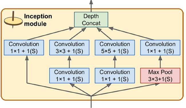
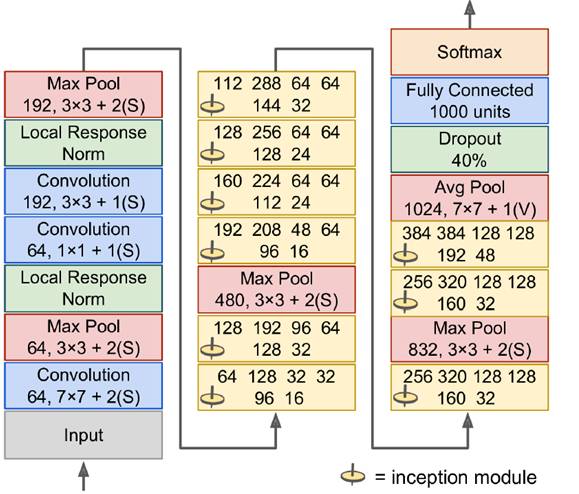
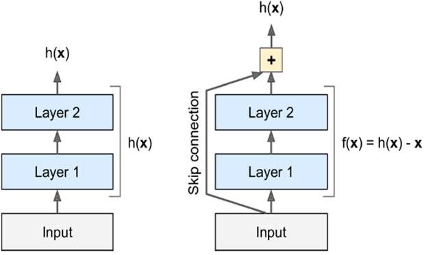
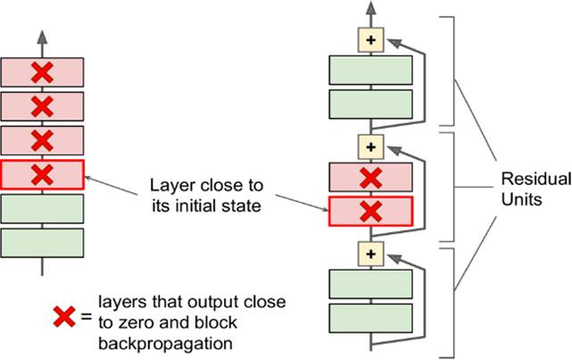
In the last century, scientists discovered several visual neurological features. The optic nerve has a local receptive field. The recognition of a whole picture is composed of multiple local recognition points. Different neurons have the ability to recognize different shapes, and the optic nerve has superposition ability. The pattern can be composed of low-level simple lines. Later, people found that the operation of the concatenation can reflect the process of optic nerve processing calculation. The LeNet-5, which was invented by LeCun in 1998, can greatly enhance the recognition effect.

This article focuses on the convolutional layer, the pooling layer, and the overall CNN structure.

Convolutional Layer Convolutional Layer

1, principle and parameters

It can simulate the nature of the local receptive field. The same layer is not fully connected, but a small block of connections. This small piece is the local receptive field. And by constructing specific convolutional neurons, it is possible to simulate the properties of different neurons stimulating different responses to different shapes. As shown in the figure below, one neuron processing a layer will form a feature map, multi-layer overlay, and the number of layers will gradually deepen.

The size of the feeling field (kernel or filter) can be regarded as fh*fw. Since the receptive field itself has the size, the feature map will continue to shrink. For the convenience of processing, the size of each layer is unchanged, so we add a value of 0 to each layer. (zero padding), to ensure that the processed feature map is the same size as the previous layer. The convolution operation between the layers is equivalent to multiplication with the position corresponding to the original pixel. As shown in the left figure below, the edges are guaranteed to be the same size when added, and the right image shows the convolve operation between each layer (if zero padding is not added).

But the above picture is just a simple example. Generally, the scanned image is a three-dimensional image (RGB). It is not a matrix, but a cube. We scan it with a three-dimensional block. The principle is the same as the above figure.

Sometimes scanning is not a sequence of sweeps, but a scan of the jump, moving 2-3 pixels each time (stride), but not completely separated will not cause information loss, so the feature map is reduced compared to the original image, to achieve The effect of information gathering.

As shown in the grayscale image below (2d), only the vertical filter is extracted on the left side, and only the horizontal filter is extracted on the right side. It can be seen that the beam is brighter and a large number of different such filters (such as can be identified) The superposition of the corners and the filter of the polyline can form multiple feature maps

The following picture is a 3d RGB effect. Each kernel (filter) can scan a feature map. Multiple filters can superimpose thick feature maps. The previous layer of filter can be convolved to form a pixel of the next layer. point.

As shown in the figure below, it can represent an output pixel value of i-line j-column k-depth, k' represents the kth filter, w represents the value in filter, x represents input, and b is a bias value.

2, TensorFlow implementation

The following is the code implemented using TensorFlow, mainly using the conv2d function

Import numpy as npfrom sklearn.datasets import load_sample_images# Load sample imagesdataset = np.array(load_sample_images().images, dtype=np.float32)# A total of 4 dimensions, channel represents the number of channels, RGB is 3batch_size, height, width, channels = Dataset.shape# Create 2 filters# General Reliance Size 7*7, 5*5, 3*3, set 2 kernels, output 2 layers feature mapfilters_test = np.zeros(shape=(7, 7, channels, 2) , dtype=np.float32)# The first (0) filter setting, 7*7 matrix, 3 is the middle filters_test[:, 3, :, 0] = 1 # vertical line# second (1) Filter setting filters_test[3, :, :, 1] = 1 # horizontal line# a graph with input X plus a convolutional layer applying the 2 filtersX = tf.placeholder(tf.float32, shape=(None, height, width , channels))# Although the input is a 4D image, since both batch_size and channel are fixed, use conv2d# strides to set, the first and fourth are both 1 to skip batch_size and channel# 2 means that the horizontal and vertical are reduced by 2, which is equivalent to reducing the entire picture to Coming to a quarter, doing a 75% reduction convolution = tf.nn.conv2d(X, filters, strides=[1,2,2,1], padding="SAME")with tf.Session() as sess : output = sess.run(convolution, feed_dict={X: dataset})

The following is the difference between the value of padding SAME and VALID (filter width is 6, stride is 5), SAME ensures that all image information is added zero padding by convolve, and VALID only adds pixels included

3, the memory calculation

Compared to the traditional fully connected layer, the convolutional layer is only partially connected, saving a lot of memory.

For example: a convolutional layer with a 5*5 size filter, outputting 200 feature maps of 150*100 size, stride takes 1 (ie no jump), and padding is SAME. The input is a 150*100 RGB image (channel=3), the total number of parameters is 200*(5*5*3+1)=15200, where +1 is bias; if the output is represented by 32-bits float ( Np.float32), then each picture will occupy 200*150*100*32=9600000bits (11.4MB). If a training batch contains 100 pictures (mini-batch=100), then this layer of convolution will Occupies 1GB of RAM.

It can be seen that training the convolutional neural network is very memory intensive, but when used, only the output of the last layer can be used.

Pooling Layer pooling layer

1, principle and parameters

When the size of the image is large, the memory consumption is huge, and the role of the Pooling Layer is to concentrate the effect and alleviate the memory pressure.

That is, a certain size area is selected, and the area is represented by a representative element. There are two specific types of lighting, taking the mean and taking the maximum. As shown in the figure below, it is a pooling layer with a maximum value. The size of the kernel is 2*2. The size of the stride depends on the size of the kernel. Here is 2, which is the value that makes all the kernels do not overlap, thus achieving efficient information compression. The original image is compressed halfway vertically and horizontally. As shown in the image to the right, the features are basically completely preserved.

The pooling operation does not affect the number of channels. Generally, the operation is not performed on the feature map (that is, the z-axis is generally unchanged), and only the horizontal and vertical sizes are changed.

2, TensorFlow implementation

# Create a graph with input X plus a max pooling layerX = tf.placeholder(tf.float32, shape=(None, height, width, channels))# Select the maximum_max_pool method# If it is the average, here is Mean_pool# ksize is the kernel size, feature map and channel are both 1, horizontal and vertical is 2max_pool = tf.nn.max_pool(X, ksize=[1,2,2,1], strides=[1,2,2,1 ],padding="VALID")with tf.Session() as sess: output = sess.run(max_pool, feed_dict={X: dataset}) overall CNN framework

Typical CNN architecture

The famous CNN architecture:

LeNet (MISIT)-1998: Input 32*32 (zero padding added to 28*28 image). The first layer of kernel uses 6 neurons, the kernel size is 5*5, stride takes 1 and the output is 28*28; the second layer does average pooling, 2*2 kernel, stride is 2, the output becomes original Half of it does not change the number of feature maps; the third layer puts 16 neurons, the other is the same; the fifth layer uses 120 neurons, and the 5*5 kernel convolves 5*5 inputs, no way Then slide, the output is 1*1; F6 connects all 84 neurons with 120 1*1 outputs, and Out connects 10 neurons, corresponding to the 10 digits of handwritten recognition output.

The tanh used in the activation function is commonly used in traditional CNN. The output layer uses RBF to be special. It is a way to calculate the distance to judge the distance between the target output and dost. .

AlexNet-2012: first used in competitions, nearly 10% improved accuracy

Enter a color image of 224*224, C1 is a large 11*11 filter, stride=4. . Finally, do a 3-layer convolution. . Finally, the classification results of 1000 classes are output.

The activation function uses ReLU, which is very popular today, and softmax for the output layer.

A little trick AlexNet uses is Local Response Normalization.

This operation adds a bias to the traditional output, taking into account some of the output effects of the neighbors. That is, if there is a very big output next to an output, its output will be paralyzed, and if it receives suppression, it can be seen that the entire term containing β is on the denominator. But later found that this technology is not very obvious for the improvement of the classifier, and some are useless.

GoogleLeNet-2014:

A large number of applications are used in the Inception module. One input comes in and is processed in four steps. After the four steps are processed, the depth is directly superimposed. Operate the picture on different scales. A large number of 1*1 convolutions can be used to flexibly control the output dimensions and reduce the number of parameters.

As shown on the right, the input is 192, using the 9-layer inception module. If you use 3*3, 5*5 parameters directly, you can count it. After that, the number of inception parameters is very large, and the depth can be adjusted. You can specify any The number of feature maps, the dimension is reduced by increasing the depth. The six parameters of the inception module correspond to the six convolutions. The above four parameters correspond to the above four convolutions. Adding the max pool does not change the number of feature maps (such as 480=128+192+96+64).

The correct rate is raised to 95-96%, which exceeds the human resolution. Because there are many kinds of dogs in image net, humans cannot distinguish them one by one.

ReSNet Residual Network-2015:

Instead of learning an objective function directly, the input directly jumps to the middle layer and directly connects to the output. To learn the residual f(x), the input skips the middle layer and directly adds it to the output.

The advantage is that the depth model path depends on the restriction that the gradient passes through all layers when it is forwarded. If there is a layer in the middle, the previous layer cannot be trained. The residual network continually jumps, even if some layers in the middle have died, the information can still flow effectively, so that the training signal is effectively transmitted back.

Area Array Sensor

Area Array Sensor,Passive Infrared Detector,Infrared Heat Detector,Infrared Area Sensor

Ningbo NaXin Perception Intelligent Technology CO., Ltd. , https://www.nicswir.com